(Re)Learning Machine Learning – Linear Regression

I am writing this as I relearn the basics of machine learning to record my thoughts and hopefully help someone (probably me) in the future. I find that I learn best when I implement the algorithms myself, even if I have to make less-efficient versions of built-in functions that many tutorials gloss over.

If you’d like to skip ahead, the full code is at the very bottom.

Environment and Requirements

I am using Python 3 with sklearn and numpy in a jupyter notebook.

For this post you’ll have to at least kind of remember calculus. Not a lot, but remind yourself what a derivative is. You should also remember how matrix math works.

Goal

What we are trying to do is predict the price of a house based on a bunch of information about the house (such as number of rooms, property tax rate, age, etc.) using linear regression. We want to use the equation for a line (the linear) to predict a real-value for the house (hence regression, as opposed to classification).

Start

You may remember that the equation for a line is:

y = m \cdot x +b

In our case, we will use w, or “weights”, instead of m. The weights can be a single value in the one-dimensional case (like below) or a vector in the multidimensional case. It can be thought of as the slope of the line we want to make. The other term is b, or “bias”, and is the offset of the line. It is where the line crosses the y-axis at x = 0. We will rewrite our equation using y-hat (the prediction we make) instead of y (the actual data we start with) and w instead of m.

\hat{y} = w \cdot x + b

In general, we are given some data that has the input (x) and output (y) and we try to make the line fit the best we can by adjusting w and b so that w*x + b is as close to y as possible. Since we have a lot of data points, we won’t be able to fit them all perfectly (which is okay and actually probably for the best!), but we’ll be able to get close. Hopefully.

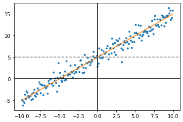
A hypothetical set of input data and the predictive line that goes with it.

In the above graph we were given the blue dots and want to make the red line. In this case the best fit line is w = 1 and b = 5, meaning the slope is 1-for-1 x-to-y and we move everything up by 5.

Since the goal is to make the line as close to all the points as possible, this means we have to be able to judge how good any version of our line is. We use a cost function to determine how good a fit any particular line is. This is called a supervised learning problem because we know the actual value of each house beforehand. We want predictions that are as close as possible to the real thing, so the further off those predictions are, the more it will cost us. The classic loss function to use here is the squared error:

cost, J(\theta) = (prediction – actual)^2

This must be repeated for every input sample, so eventually the cost will be the average over all the samples, making it the mean squared-error, or MSE.

Gradient Descent

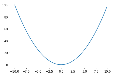
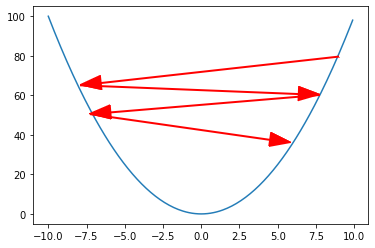
Finally, we need to know how to update the weights. You can think of the cost function as some hilly field that you could walk on. Minimizing the cost function is like finding the lowest point on the field. How do you know which direction is downhill? You can use derivatives to find out what the slope (gradient) is where you’re standing, and then go downwards (descent).

This is what the cost function looks like. We want to get to the bottom!

The derivative of the cost function will require using the chain rule. We will first get the partial derivative with respect to w. This is like if I wanted to see where down was in the North-South direction, and then the next partial derivative would be seeing which way was down in the East-West direction. Here, we will say the cost function is a function of θ, which has both w and b in it.

\begin{aligned} {\frac d {dw} J(\theta)}& = {\frac {d} {dw} }(prediction – actual)^2 \\ &= {\frac {d} {dw} }(w x + b – y)^2 &&\text{power rule}\\ &= 2(w x + b – y) \cdot {\frac {d} {dw} }(w x + b – y) &&\text{chain rule}\\ &= 2(w x + b – y) \cdot x &&\text{multiplication by constant}\\ &= 2x(w x + b – y) &&\text{gather terms}\\ &\text{where } \hat{y} = wx+b,\\ & = 2x(\hat{y} – y) \\ &\text{so, over all } m \text{ training examples,}\\ {\frac d {dw} J(\theta)} &= \frac{1}{m} 2x\displaystyle\sum_{i=1}^m (\hat{y}-y) \end{aligned}

This is where you have to remember calculus. The chain rule states that d/dx of f(g(x)) is f'(g(x))*g'(x), and in this case f(x) = x^2 and g(x) = wx+b-y. The power rule says d/dx of x^n = n*x^(n-1), so x^2 goes to 2x. The derivative of x*C, where C is a constant, is C. This basic idea works for any number of weights in w, since they are all independent of each other. They will all have the same form (except they’ll be w_1, w_2, etc.)

Next is for d/db, which follows the same process:

\begin{aligned} {\frac d {db} J(\theta)} &= {\frac {d} {db} }(w x + b – y)^2 \\ &= 2(w x + b – y) \cdot {\frac {d} {db} }(w x + b – y) \\ &= 2(w x + b – y) \\ &\text{where } \hat{y} = wx+b,\\ & = 2(\hat{y} – y) \\ &\text{so, over all } m \text{ training examples,}\\ {\frac d {db} J(\theta)} &= \frac{1}{m} 2\displaystyle\sum_{i=1}^m (\hat{y}-y) \end{aligned}

Now we have the gradient (direction) we want to go for each variable. We would just subtract d/dw and d/db from w and b, respectively. Just repeat this step a bunch of times and eventually you’ll get your weights and bias that you can use to make predictions.

Again, this is the cost for a single sample, so you’ll need to sum up and average across all input samples when making the real thing.

The code

First, downloading the dataset:

There are a couple other parts to the dataset, including description, but for the purposes of learning linear regression they are not important. The data will come in as a m x n matrix, with m being the number of examples and n being the number of features. Basically, each row is a sample and each column is a feature type. Below is a graph of the number of rooms vs. value of the house:

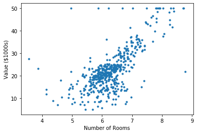
You could draw a straight line that follows the dots pretty well, meaning that there’s a pretty good linear relationship between number of rooms and the value of a house and our model should work.

Next we wanna implement gradient descent. We want to figure out which direction and how far to step, then repeat. The following code does one update:

First it resets the gradient to zero, then it loops through each training example. For each example, it makes a prediction, then uses the update function we derived above to get the gradient for each variable. Then, we update the variables by the average value of the derivative across all training examples. In other words, for each input example we figure out which way is down and how steep it is, then we find the average value for that across all examples and move in that direction.

The following is the main portion of the program:

First we initialize our data and weights. Weight initialization is a topic in and of itself. Here we’re just going to use all zeros, but for other algorithms you might not want to use zeros (such as initializing neural network weights). All zeros will work here so for now we just won’t think about it.

Next is “alpha”, or the learning rate. This affects how big of a step your algorithm takes when updating the weights. Too small of a learning rate and the algorithm will take forever. Too large and it will take large leaps and jump around the cost function from side to side without ever reaching the bottom.

This might happen if alpha is too large. Each step the algorithm takes is too large, overshooting the minimum each time.

Actually running the code

If you try to run the code as is, you might notice a few things. First, it might not work at all if you’re using more than one feature. The cost function will explode larger and larger until you get an overflow error. Oops.

This is likely due to the fact that the different features are at different scales which messes up the gradient calculation. In other words, number of rooms is anywhere from 0 to 100, but another feature (like proportion of residential land zoned for lots over 25,000 sq ft) may only go from 0 to 1, and when you try to look at them together it doesn’t work very well.

The solution is to normalize the input data. The following code is a neat trick using lambdas to make a reversible change to the data set.

For each feature, it finds the min and max, then transforms every point to fit in the (0,1) range. They key equation is:

x_{transformed} = (x – min(x))/range(x)

You want to apply this one feature at a time across the entire sample. You need to get the max value, the min value, then apply this equation to each entry. The max and min value can be taken from the samples themselves or from an arbitrary range. It uses the transformMaker() function and untransformMaker() function to store a function to do or undo the transform. You’ll need to reproduce the transform when you get new data and you might need to untransform just in case.

The second thing that can be improved is through using vectorized calculations. Every prediction can be made in a single step without looping by doing a matrix multiplication. This is much faster and gives the same result because each prediction only depends on one example. The gradients can be calculated in a single step in a similar manner. The following is the vectorized version of update and avg_loss(), a function to calculate the average loss:

No loops, and much faster! You may notice that I’m using x.T for calculations. Our weight vector, w, is of size (13,). Notice the comma, that means it only has one dimension. Numpy will let us be lazy and use it for np.matmul(). For our prediction vector, we want to end up with a m x 1 vector, where m is the number of input samples, so we need to make the multiplication with x end up with those dimensions. A reminder about matrix multiplication, the inner two dimensions need to match. You can multiply a 1 x 10 vector with a 10 x 10 matrix, but not a 1 x 7 vector with a 10 x 10 matrix. Secondly, the dimensions of the resulting vector will be the outer dimensions of the two inputs. A 1 x 10 vector and 10 x 7 matrix will make a 1 x 7 matrix.

The input data, x, is a m x 13 matrix (each row is a sample). Since we’re looking for a 1 x m prediction vector, we will multiply w (1 x 13) with the transpose of x (13 x m).

For dw we do the same thing. Again, numpy is nice and lets us be lazy with multiplying matrices with vectors using matmul(), so we just need to make sure that the 13 is on the outside, resulting in a 13 x 1 vector for dw. The sum across samples happens as a part of the matrix multiplication.

Caveats

Normally you’d want to do things like set aside a training/validation/test set or do cross validation, or any number of other analytic techniques, but the purpose of this post is to learn linear regression, not carry out an entire data science project. We just want to use linear regression and gradient descent to find weights to fit the data.