(Re)Learning Machine Learning – Logistic Regression

This time we’re going to do logistic regression. Logistic regression uses the same idea as linear regression (see my previous post) to classify input as one of two different classes. Instead of a linear function (one that looks like a straight line) we use a log-based function (making it “logistic”), and even though we’re using it to classify, since it has the same idea as linear regression, we still call it “regression”.

Environment and Requirements

I’ll be using Python 3 with numpy and sklearn in a jupyter notebook. I will also be using matplotlib later on for displaying the results (it’s also how I made all these graphs!).

Same as before, you should remember some calculus, linear algebra (specifically derivatives and matrix math), and what a logarithm is.

Goal

The goal of logistic regression is to categorize something as one of two classes. For example, we might want to know if a cookie is M&M or dark chocolate chip. Every bite we take has a set of features (color, flavor, texture, etc.). The strategy is to take these features, then pass them through a function that gives us a value between 0 (M&M cookie) and 1 (dark chocolate chip). The closer to 1, the more certain we are it is chocolate chip. The closer to 0, the more certain we are it is M&M.

Start

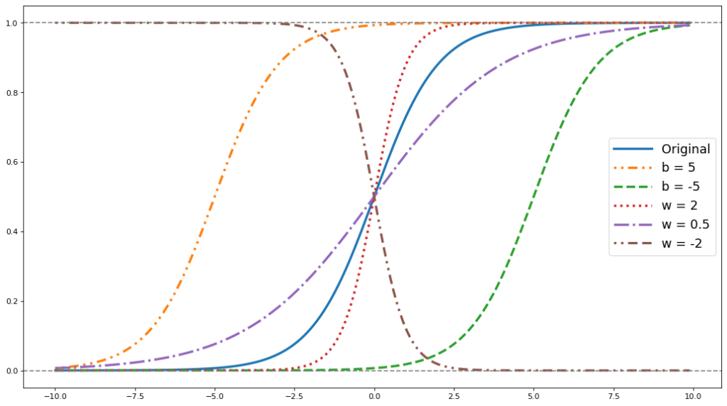
So, we need a way to map our input (which can be any real number) to the range (0,1). One function that is used to do this mapping is the sigmoid, or σ(x). The basic form is:

\text{Sigmoid, } \sigma(x) = \frac {1}{1+e^{-(wx+b)}}

This curve can be stretched and changed using the weights, w, and the bias, b. The following graph has examples of sigmoids with different weights:

Training data comes in as an input x and its corresponding class. Because we know what the correct answers are supposed to be, this is a supervised learning problem. With our cookie example of M&M cookie vs dark chocolate chip, each input x might be a single nibble of one cookie. We might get something like this:

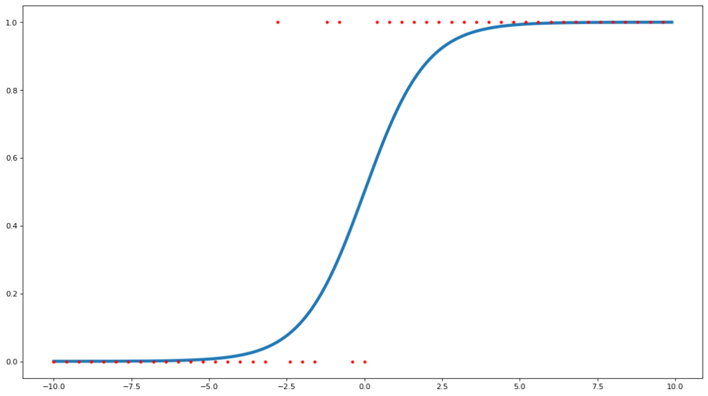
The red dots are the cookies and they are either 0 (M&M) or 1 (dark chocolate chip). The x-axis is the level of chocolateyness, with -10 being sweet chocolate, 0 being no chocolate, and 10 being ultra dark chocolate. The blue line is the sigmoid function fitted to the input data, your rule on judging the cookies based on the chocolate flavor. Sometimes you get a bite of that sweet M&M flavor, represented by x = -10, and you’re absolutely sure that this cookie is an M&M cookie (σ(x) = 0, the chance this was dark chocolate chip = 0). Sometimes you get a bite with rich dark chocolate (x = 10) that is unmistakably the dark chocolate chip (σ(x) = 1, 100% chance this was dark chocolate chip). Sometimes, you don’t get any chocolate at all (x = 0), so you’re not quite sure which one it is (σ(x) = 0.5, or a 50/50 chance) , but sometimes those bites came from an M&M cookie and sometimes they came from a dark chocolate chip cookie (some red dots around x=0 are at 1 and others are at 0).

So where do we proceed from here? We can use gradient descent, like we did with linear regression, but this time instead of mean squared-error we will use maximum likelihood estimation.

Gradient Descent

For gradient descent, we will need to use a cost function, J(x). When we did linear regression, we used the average squared distance (also known as mean squared-error, or MSE) between our prediction and the target as our cost function. This works well when the target can be any real number, but here it is not a good choice. First, the target can only be a 0 or a 1. Second, and more importantly, mean squared-error is non-convex for logistic regression. For linear regression, the cost function using MSE was a parabola and there were no “fake-bottoms”, or local minima, to the curve where we might get stuck. It was a convex function. This is not the case when using the sigmoid function for logistic regression.

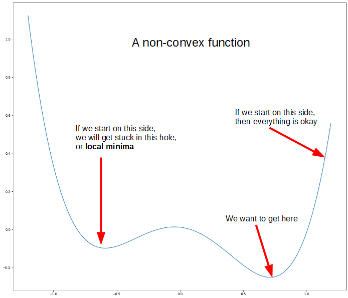
Optimizing the cost function is kind of like dropping a marble, and the goal is to get to the bottom. If we imagine that the above graph was our cost function, we can see we’re not always guaranteed to get to the bottom. The problem here is that we don’t know exactly where we’ll start when we initialize the algorithm. If we drop the marble on the right side, then we’re safe and we’ll reach the bottom no problem. If we drop the marble on the left side, then we’ll probably get stuck in that hole and won’t be able to get out (note: there are some workarounds to this such as simulated annealing)

The proof for that will need another post, but it involves taking the second derivative of the cost function. The first derivative shows you the slope of the function, the second derivative shows the change in slope. For example, if you are driving home and x is your distance from home, then the first derivative would be your speed, or how fast x is changing. The second derivative would be acceleration, or how fast your speed is changing.

Instead, we will use:

Maximum Likelihood Estimation (MLE)

Maximum likelihood estimation tries to find the parameter values that maximize the likelihood of this data. This way of thinking might be the way you as a human try to solve certain problems. For example, let’s say your jerk of a roommate likes to play darts using a thin piece of paper on the wall as their dartboard. You can tell where the bullseye was by using the pattern of holes in the wall. You might think to yourself, “Given that the holes are mostly centered around this spot, I’m guessing this is where you put the target”.

MLE uses much the same idea. “What are the parameters that are most likely to give this data that we have?”

A Primer on Probability

Probability is the chance that an event will happen. If I have a fair coin, then there’s a 50/50 chance it will land heads or tails. Each has a 50% probability, that is P(H) = P(T) = 1/2. What are the chances that I flip a heads and then a tails? Well, since this is a fair coin and every flip is independent, meaning it doesn’t affect any other flip, the probability of getting exactly heads then tails is P(H) × P(T) = 1/2 × 1/2 = 1/4, or 25%. You can continue this to any number of coinflips, multiplying together each time.

I won’t go much deeper, but I will have a post that covers the basics more thoroughly.

Back to MLE

So what are we trying to do during MLE? We are trying to maximize likelihood. We are trying to say, given the data we see here, what are the most likely parameter values? In other words, we want to maximize the likelihood of the data. Recall that σ(x) is the likelihood that x is class 1, therefore we want to maximize σ(x) when the answer, y = 1. The complement, 1 – σ(x), is the likelihood that x is class 0, so we’ll try to maximize that when y = 0. Our likelihood function is now:

L(\theta|x) = \begin{cases} \sigma(x) &\text{if y=1}\\ 1-\sigma(x) &\text{if y=0} \end{cases}

We can write this in a slightly different way

L(\theta|x) = \sigma(x)^y × (1-\sigma(x))^{(1-y)}

When y = 1, L(θ|x) = σ(x) × (1 – σ(x))^0 = σ(x), and when y = 0, L(θ|x) = σ(x)^0 × (1 – σ(x))^1 = 1 – σ(x).

To get the total probability over all x, we multiply their individual probabilities together (just like when we were getting the total probability for multiple coin flips). Here, X represents all samples, or the whole training set. You might also see the product operator, represented by Π, a capital pi. Where capital sigma, Σ, is the sum of the elements, capital pi Π is the product of all the elements.

L(\theta|X) = \displaystyle\prod_{i=1}^{m}\sigma(x_i)^y (1-\sigma(x_i))^{1-y}

Although this is perfectly fine, this form of the equation won’t work well when we’re actually computing the probabilities because of the limits of computing extremely small decimals on a computer. Instead, we will transform this using a logarithm to create the log-likelihood. Doing this transformation doesn’t affect our results because the logarithm is a monotonically increasing for positive real numbers (there are no negative probabilities). This means that for all values of the input x, as you increase x the f(x) also increases. Since we’re trying to maximize L(θ|x), we’ll get the same answer if we maximize log(L(θ|x)), as whatever maximizes one will maximize the other.

Here is what the log-likelihood looks like:

LL(\theta|X) = \displaystyle\sum_{i=1}^{m} y \ln(\sigma(x_i))+ (1-y)\ln(1-\sigma(x_i)) \\ or\\ LL(\theta|x) = \begin{cases} \ln(\sigma(x)) &\text{if y=1}\\ \ln(1-\sigma(x)) &\text{if y=0} \end{cases}

Gradient Descent vs Ascent

If we were to use the log-likelihood as-is, we’d have to use a gradient ascent algorithm instead of gradient descent like with linear regression. It’s basically the same thing, except we flip a sign to make it go the other direction. Easy peasy lemon squeezy!

So, if you want to use the log likelihood as a cost function for gradient descent, just flip the signs:

\text{Let } \hat{y} = \sigma(x)\\ J(x) = -y \cdot \ln(\hat{y}) -(1-y)\cdot \ln(1-\hat{y})\\ or\\ J(x) = \begin{cases}-\ln(\hat{y} ) &\text{if y=1}\\ -\ln(1 – \hat{y} ) &\text{if y=0} \end{cases}

What does this actually mean?

Why does this work? What does it mean? Back to our cookie example: if we had actually grabbed a dark chocolate chip cookie (class 1), then we want to have the highest cost for guessing M&M (class 0). If we are 10% sure it’s dark chocolate chip when it actually is chocolate chip then the guess costs us -log(.1) = 2.3. If we are 60% sure it’s chocolate chip when it actually is chocolate chip, then our guess only cost us -log(0.6) = 0.51. The loss function ends up looking like this:

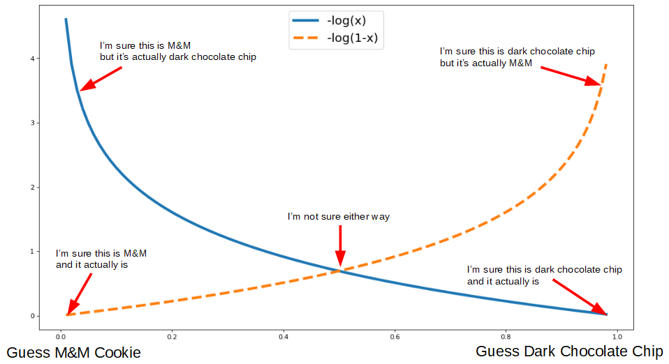
It the current bite was actually from a dark chocolate chip cookie (class 1), then we use the solid blue line (-log(x)), and going “down” means moving towards classifying this as a 1. If the current bite was actualy from an M&M cookie (class 0), then we use the dashed orange line (-log(1-x)), and going “down” means moving towards classifying this as a 0. The compact way of writing this loss function is:

If y=1, then we use only the left half because the (1-y)=0 and cancels the right half. If y=0, same thing happens but in the other direction.

DANGER: MATH AHEAD

I will be deriving the equations for dw and db, so feel free to jump ahead to the answer.

Next, we must derive dw and db for use in our gradient descent algorithm. First, we’ll find the derivative for the sigmoid function σ(x). (I had help for this step). Note, θ includes both w and b.

First we’ll do a small derivative that will help us keep things neat later:

\begin{aligned} g(\theta) &= 1 + e^{-(wx+b)}\\ \frac{d}{dw}g(\theta) &=-x\cdot e^{-(wx+b)} = -x (1-1+e^{-(wx+b)}) = -x (1-g(\theta))\\ \frac{d}{db}g(\theta) &=-e^{-(wx+b)} = 1-1+e^{-(wx +b)} = 1-g(\theta) \end{aligned}

Next, we will find the partial derivatives for σ(x). Note that the process almost identical for dw and db, so I’ll only go through the steps for dw.

\begin{aligned} \sigma(x) &= \frac{1}{1+e^{-(wx+b)}} = \frac{1}{g(\theta)}\\ \frac{d}{dw}\sigma(x) &= \frac{(0)g(\theta) – (1)g'(\theta)} {g(\theta)^2} &&\text{quotient rule} \\ &= \frac {g'(\theta)} {g(\theta)^2}=\frac{-x(1-g(\theta))} {g(\theta)^2} &&\text{simplify/substitue} \\ &= = -x\frac{1-g(\theta)} {g(\theta)^2}=-x\bigg(\frac{1}{g(\theta)^2} – \frac{g(\theta)}{g(\theta)^2}\bigg)&&\text{some algebra}\\ \\ &= -x \frac{1}{g(\theta)} \bigg( \frac{1}{g(\theta)} – \frac{g(\theta)}{g(\theta)}\bigg)&&\text{pull out}\frac{1}{g(\theta)}\\ &=-x\sigma(x)(\sigma(x) – 1) &&\text{substitute} \\ &= x \sigma(x) \big( 1 – \sigma(x) \big) \\ &\text{Follow the same pattern for}\space \frac{d}{db}\sigma(x) \space \text{to get} \\ \frac{d}{db} \sigma(x)&= \sigma(x)(1 – \sigma(x)) \end{aligned}

Now, lets work on the cost function. For ease of derivation, we’re going to use the natural log, because the derivative of ln(x) is 1/(x).

\begin{aligned} J(\theta) &= -y \cdot ln\big( \sigma(x) \big) – (1-y)\cdot ln\big( 1- \sigma(x) \big) \\ \frac{d}{dw}J(\theta)&=\bigg[ -y \frac{1}{\sigma(x)} \cdot \sigma'(x) \bigg] – \bigg[ (1-y) \cdot \frac{1}{1-\sigma(x) }\cdot -\sigma'(x) \bigg] &&\text{chain rule} \\ & = \bigg[-y \cdot \frac{1}{\sigma(x)}\cdot x \sigma(x)(1 – \sigma(x)) \bigg] – &&\text{substitute} \\& \hspace{5pc} \bigg[(1-y) \cdot \frac{1}{1-\sigma(x)} \cdot -x \sigma(x)(1-\sigma(x)) \bigg] \\ & = \Big[-xy(1-\sigma(x))\Big] – \Big[ -x\sigma(x)(1-y) \Big] &&\text{simplify}\\ &= \Big[-xy+xy \sigma(x)\Big] -\Big[-x\sigma(x) +xy\sigma(x)\Big] && \text{distribute}\\ & = -xy + x\sigma(x) &&\text{simplify}\\ & = x\hat{y} – xy &&\hat{y} = \sigma(x) \end{aligned}

So, over all m training examples, the update rule becomes:

\begin{aligned} \frac{d}{dw}J(\theta)&= \frac{1}{m}\displaystyle\sum_{i=1}^m x_i\Big(\hat{y} – y\Big) \\ \frac{d}{db}J(\theta)&= \frac{1}{m} \displaystyle\sum_{i=1}^m \Big(\hat{y} – y\Big) \end{aligned}

Wow. All that work and it looks pretty much like the update rule from linear regression.

So, now that we have the parameter values (sometimes called beta values), how do we actually use them?

The actual strategy

Now that we have descended upon a good set of weights, how do we actually use them? We use them in the following equation:

y = b + \sum_{i=1}^n{w_ix_i} \newline \text{Our guess} = \sigma(y)

For a given input sample, we multiply each feature by its corresponding weight, add the bias term (if any), and then put the result into the sigmoid function. The sigmoid will push y to be in the ‘S’ shape we saw above and it will have a value from 0 to 1. We can use this value as the probability this sample is of class 1, or in other words, the probability that this cookie is dark chocolate chip.

Now on to the code.

The Code

First, we will do our imports, load the data, and create the transforms for normalizing each feature. The two functions, untrasformMaker() and transformMaker(), are for (de)normalizing the data in case, for example, we get new data and want to run it through the model. As I talked about during my linear regression post, normalizing the data helps make your gradient descent run smoothly.

Next, is the sigmoid and update functions:

The sigmoid, as above, follows the equation from above, and returns a 1 x m vector of values. The update function get the prediction based on the current parameters using sigmoid(). Then, following the update rules we derived above, we calculate the sum across all input samples. Finally, we update the parameters by taking the mean and applying the learning rate, α.

When determining accuracy, we first get our prediction model, which gives us the probability that this sample is class 1. A high value means it his highly likely class 1. Instead of just saying anything over 0.5 is class 1 (which is a valid choice in certain circumstances), I will use this prediction as the probability of class 1. For example, if x = -.3, σ(x) = 0.7, that means we have a 70% chance of classifying this sample as class 1. We generate a random number from 0 to 1, and if it’s less than σ(x), then we say this sample is class 1.

The main loop is as follows:

We grab the data we want (we can optionally grab a single feature), then initialize the parameters, then loop over the update. As a little upgrade over the linear regression, I added a variable to track the history of the model, mostly to see how accuracy improves over time. In order to see this, we can use matplotlib, a nifty plotting module.

This results in the following graph:

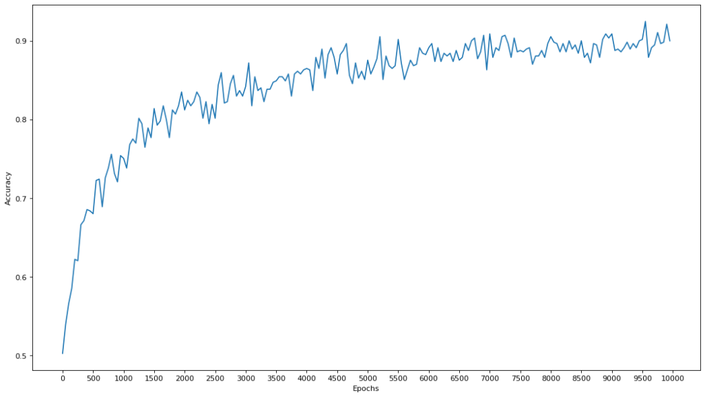
Here we see the accuracy of the model over every loop (epoch). We start at 50% accuracy (randomly guessing between two choices) and then rapidly improve.

As you can see, we reach up to about 90% accuracy in classifying the input data. Pretty good! The reason why it fluctuates a lot is because of the way we used the model as a probabilistic predictor, not an absolute one. If we said that if the model predicts over 0.5 then classify it as 1 always, we would get a similar but much more blocky shape.

Caveats

Of course, since we’re using the entire data set it’s most likely overfitting to the training data and the actual performance would not be this good. Normally you’d do things like split the data into training/validation/test sets or do cross-validation, but that is out of the scope for this post. All we want to do right now is learn logistic regression, we can save learning about training procedures for another post.